Tamilnadu State Board New Syllabus Samacheer Kalvi 12th Business Maths Guide Pdf Chapter 8 Sampling Techniques and Statistical Inference Miscellaneous Problems Text Book Back Questions and Answers, Notes.
Tamilnadu Samacheer Kalvi 12th Business Maths Solutions Chapter 8 Sampling Techniques and Statistical Inference Miscellaneous Problems
Question 1.
Explain the types of sampling.
Solution:
There are two types of sampling. They are
(1) Non-Random sampling or Non-probability sampling
(2) Random sampling or probability sampling Random sampling refers to selection of samples from the population in a random manner. A random sample is one where each and every item in the population has an equal chance of being selected.
“Every member of a parent population has had equal chances of being included “Dr. Yates.
“A random sample is a sample selected in such a way that every item in the population has an equal chance of being included”-Harver.
The different types of probability sampling are
(1) sampling random sampling
(2) stratified random sampling
(3) systematic sampling
![]()
Question 2.
Write short note on sampling distribution and standard error.
Solution:
sampling distribution:
Sampling distribution of a statistic is the frequency distribution which is formed with various values of a statistic computed from different samples of the same size drawn from the same population.
For instance if we draw a sample a size n from a given finite population of N, then the total number of possible samples is
Ncn = \(\frac { N! }{n!(N-n)!}\) = k(say)
Standard Error:
The standard deviation of the sampling distribution of a statistic is known as its standard Error abbreviated as S.E. The standard Error (S.E) of some of the well-known statistics, for large samples, are given below, where n is the samples size, σ² is the population variance.
![]()
Question 3.
Explain the procedures of testing of hypothesis
Solution:
The following are the steps involved in hypothesis testing problems:
1. Null hypothesis: Set up the null hypothesis H0
2. Alternative hypothesis: Set up the alternative hypothesis. This will enable us to decide whether we have to use two tailed test or single tailed test (right or left tailed)
3. Level of significance: Choose the appropriate level of significant (a) depending on the reliability of the estimates and permissible risk. This is to be fixed before sample is drawn, i.e., a is fixed in advance.
4. Test statistic : Compute the test statistic
Z = \(\frac { t-E(t) }{\sqrt{var(t)}}\) = \(\frac { t-E(t) }{S.E(t)}\) N(0, 1) as n → ∞
5. Conclusion: We compare the computed value of Z in step 4 with the significant value or critical value or table value Zα at the given level of significance.
(i) If |Z | < Zα i.e., if the calculated value of is less than critical value we say it is not significant. This may due to fluctuations of sampling and sample data do not provide us sufficient evidence against the null hypothesis which may therefore be accepted.
(ii) If |Z |> Zα i.e., if the calculated value of Z is greater than critical value Zα then we say it is significant and the null hypothesis is rejected at level of significance α.
![]()
Question 4.
Explain in detail about the test of significance for single mean.
Solution:
Let xi , (i = 1, 2, 3, …, n) is a random sample of size from a normal population with mean µ and variance σ² then the sample mean is distributed normally with mean and variance
\(\frac { σ^2 }{n}\), i.e \(\bar { x }\) N(µ, \(\frac { σ^2 }{n}\))
Thus for large samples, the standard normal variate corresponding to \(\bar { x }\) is
Z = \(\frac {\bar { x } -µ }{\frac{σ}{√n}}\) N (0, 1)
Under the null hypothesis that the sample has been drawn from a population with mean and variance σ², i.e., there is no significant difference between the sample mean (\(\bar { x }\)) and the population mean (α), the test statistic (for large samples) is:
Z = \(\frac {\bar { x } -µ }{\frac{σ}{√n}}\)
Question 5.
Determine the standard error of proportion for a random sample of 500 pineapples was taken from a large consignment and 65 were found to be bad?
Solution:
sample size n = 500
No. of bad pine apples = 65
sample proportion = P = \(\frac { 65 }{500}\) = 0.13
Q = 1 – p ⇒ Q = 1 – 0.13
∴ Q = 0.87
The S.E for sample proportion is given by
S.E = \(\sqrt{\frac { PQ }{N}}\) = \(\sqrt{\frac { (0.13)(0.87) }{500}}\)
= \(\sqrt{\frac { 0.1131 }{500}}\) = \(\sqrt{0.0002262}\)
= 0.01504
∴ S.E = 0.015
Hence the standard error for sample proportion is S.E = 0.015
![]()
Question 6.
A sample of 100 students are drawn from a school The mean weight and variance of the sample are 67.45 kg and 9 kg respectively find (a) 95% and (b) 66% confidence intervals for estimating the mean weight of the students.
Solution:
sample size n = 100
The sample mean = \(\bar { x }\) = 67.45
The sample variance S² = 9
The sample standard deviation S = 3
S.E = \(\frac { S }{√n}\) = \(\frac { 3 }{\sqrt{100}}\) = \(\frac { 3 }{10}\) = 0.3
(a) The 95% confidence limits for µ are given by
\(\bar { x }\) – z\(\frac { α }{2}\) S.E < µ < \(\bar { x }\) + z\(\frac { α }{2}\) S.E
67.45 – (1.96 × 0.3) ≤ µ ≤ 67.45 + (1.96 × 0.3) 67.45 – 0.588 ≤ µ ≤ 67.45 + 0.588
66.862 ≤ µ ≤ 68.038
The confidential limits is (66.86, 68.04)
(b) The 99% confidence limits for estimating µ are given by
\(\bar { x }\) – z\(\frac { α }{2}\) S.E ≤ µ ≤ \(\bar { x }\) + z\(\frac { α }{2}\) S.E
67.45 – (2.58 × 0.3) ≤ µ ≤ 67.45 + (2.58 × 0.3)
67.45 – 0.774 ≤ µ ≤ 67.45 + 0.774
66.676 ≤ µ ≤ 68.224
∴ The 99% confidence limits is (66.68, 68.22)
![]()
Question 7.
The mean I.Q of a sample of 1600 children was 99. it is likely that this was a random sample from a population with mean I.Q 100 and standard deviation 15? (Test at 5% level of significance)
Solution:
sample size n = 1600
\(\bar { x }\) = 99
sample mean
Population mean µ = 100
population S.D σ = 15
under the Null hypothesis H0 : µ = 100
Alternative hypothesis H1 : µ = 100 (two tails)
Level of significance µ = 0.05
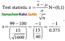
z = -2.666
z = -2.67
Calculated value |z| = 2.67
critical value at 5% level of significance is
z\(\frac { α }{2}\) = 1.96
Inference:
Since the calculated value is greater than table value i.e z ⇒ z\(\frac { α }{2}\) at 5% level of significance, the null hypothesis is rejected. Therefore we conclude that the sample mean differs, significantly from the population mean.
![]()